SPlit.jl
Distribution-preserving subset selection for tabular data and embeddings, grown from SPlit (Joseph and Vakayil, 2022): optimal train/test splits, k-fold multiplets, and training-data selection by support points, kernel herding, twinning, and kernel thinning.
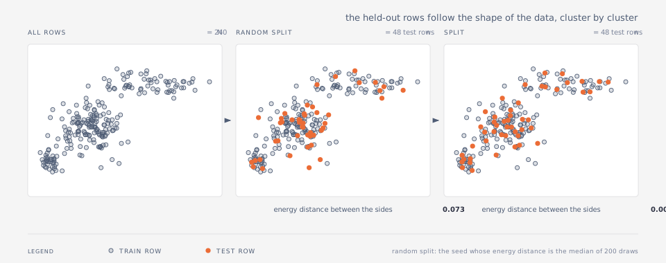
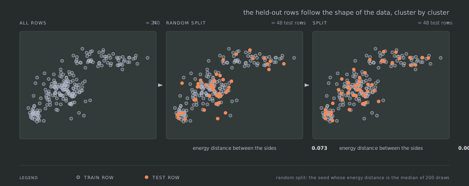
The figure is a real run on 240 two-dimensional rows: a random 20% test draw lands unevenly across the three clusters, while the rows datasplit holds out follow the shape of the data, and the energy distance between the two sides drops by more than an order of magnitude.
Overview
SPlit.jl chooses rows whose empirical distribution stays as close as possible to a target measure, under the energy distance or the maximum mean discrepancy. Three choices make up a call:
- What you get.
datasplitreturns a train/test partition,multipletreturnskdistribution-balanced folds (k= number of folds), andselectrowsreturns just thenchosen row indices (n= number of rows selected). - What you match. The data's own distribution by default;
weightsmatches a quality-weighted version of it,referencematches a separate target sample while still drawing rows from the data. - How rows are chosen.
SupportPointSplitter,HerdingSplitter,TwinningSplitter, orKernelThinningSplitter; see Methods and Benchmarks for how they differ.
The original method is SPlit: it computes support points, the sample of a given size that minimizes the energy distance to the full data (Mak & Joseph, 2018), and maps each support point to its nearest unclaimed data row (Joseph & Vakayil, 2022). Unlike random splitting, this makes both the train and test distributions close to the population distribution, which improves the reliability of model evaluation. The other three splitters select rows directly, without the continuous optimization step.
The rows need not be tabular: standardize = false passes a numeric matrix through unchanged, which is what Selecting LLM training data uses on embedding matrices.
The package also implements the optimal split ratio result of Joseph (2022): for a linear model with p parameters, the test fraction that minimizes the variance of the fitted model is γ = 1 / (√p + 1).
New to support points? Read How SPlit works first.
Quick start
using SPlit, Random

data = randn(MersenneTwister(1), 1_000, 3)

# a train/test split
splitter = SupportPointSplitter(ratio = 0.2, rng = MersenneTwister(2))
result = datasplit(splitter, data)
train = data[result, :train]
test = data[result, :test]
splitquality(data, result)                 # energy distance, lower is better
optimal_split_ratio(data[:, 1:2], data[:, 3])

# a selection: 100 rows that stand in for the whole dataset
idx = selectrows(HerdingSplitter(), data, 100)

target_sample = randn(MersenneTwister(4), 50, 3)
# rows of data that match target_sample's distribution instead of data's own
idx_target = selectrows(SupportPointSplitter(), data, 100; reference = target_sample)

# embeddings: use the rows as they are, with no per-column standardization
embeddings = randn(MersenneTwister(5), 200, 16)   # rows already on the scale you want to keep
idx_embed = selectrows(HerdingSplitter(), embeddings, 50; standardize = false)
Kernels and splitters
SupportPointSplitter accepts any SplitKernel. The default, EnergyKernel, minimizes the energy distance of Mak & Joseph (2018). GaussianKernel minimizes the squared maximum mean discrepancy (MMD², Gretton et al., 2012) instead, by projected gradient descent with Armijo backtracking (full data; kappa, the size of the per-iteration random subsample, runs a mean-shift MM, or majorization-minimization, sweep on subsamples); see Methods for both objectives.
gauss = SupportPointSplitter(kernel = GaussianKernel(), rng = MersenneTwister(3))
result = datasplit(gauss, data)
result.method.kernel            # GaussianKernel with the resolved bandwidth
splitquality(data, result; kernel = result.method.kernel)   # MMD under the fitted kernel
HerdingSplitter builds the smaller subset directly by greedy kernel herding (Chen, Welling & Smola, 2010) instead of computing support points:
herd = HerdingSplitter(kernel = GaussianKernel())   # deterministic, optimizer-free
result = datasplit(herd, data)
TwinningSplitter (Vakayil & Joseph, 2022) needs neither a kernel nor an optimizer: it chains nearest-neighbor groups through the data and keeps one row per group, in O(pN log N) (N = number of rows, p = number of columns). multiplet turns any splitter into k distribution-balanced folds:
result = datasplit(TwinningSplitter(), data)          # deterministic, energy distance
folds = multiplet(TwinningSplitter(), data, 5)        # 5 folds, sizes within one row
KernelThinningSplitter (Dwivedi & Mackey, 2022, 2024) also selects rows directly: KT-SPLIT (KT = kernel thinning) halves a shuffled sequence of rows into candidate subsets by randomized kernel halving, and KT-SWAP keeps the candidate closest to the target measure and refines it by single-row swaps, with a high-probability MMD guarantee neither HerdingSplitter nor TwinningSplitter has:
kt = KernelThinningSplitter(kernel = EnergyKernel(), rng = MersenneTwister(4))
result = datasplit(kt, data)
See Benchmarks for how the four splitters compare across kernels and dataset sizes.
Quality diagnostics
energydistance/mmd accept an estimator keyword for large inputs. See Methods for what each DiscrepancyEstimator computes:
energydistance(X, Y; estimator = RandomSlices(256))
mmd(X, Y, GaussianKernel(1.0); estimator = RandomFeatures(2048))
API reference
See the Reference section for complete API documentation.
Algorithm details
- Preprocessing. Categorical columns are Helmert-encoded, constant columns are dropped, and every remaining column is standardized to mean 0 and variance 1.
standardize = falseskips this step and uses the numeric matrix as it is. - Support-point computation. The kernel's majorization-minimization update moves a candidate point set, sweep by sweep, to minimize its energy distance to the data (Mak & Joseph, 2018). For large
n,kappaswitches to the stochastic variant that resamples rows each iteration. UnderGaussianKernelthe optimizer is projected gradient descent on the squared MMD instead (full data;kapparuns a mean-shift MM sweep on subsamples); see Methods. - Nearest-neighbor assignment. Each support point claims its nearest unclaimed data row via a k-d tree (a space-partitioning search tree; Joseph & Vakayil, 2022).
- Partitioning. The claimed rows form the smaller subset and the rest form the larger one;
ratiodecides which of the two is the test set.
Planned work and its ordering are on the Roadmap page.
References
Joseph, V. R., & Vakayil, A. (2022). SPlit: An Optimal Method for Data Splitting. Technometrics, 64(2), 166-176. DOI
Mak, S., & Joseph, V. R. (2018). Support points. The Annals of Statistics, 46(6A), 2562-2592.
Joseph, V. R. (2022). Optimal Ratio for Data Splitting. Statistical Analysis and Data Mining: The ASA Data Science Journal, 15(4), 531-538.
Gretton, A., Borgwardt, K. M., Rasch, M. J., Schölkopf, B., & Smola, A. (2012). A Kernel Two-Sample Test. Journal of Machine Learning Research, 13, 723-773.
Chen, Y., Welling, M., & Smola, A. (2010). Super-Samples from Kernel Herding. UAI, 109-116.
Rahimi, A., & Recht, B. (2007). Random Features for Large-Scale Kernel Machines. NIPS, 20.