Methods
See How SPlit works for the same quantities explained with analogies instead of formulas.
This page first walks through the procedure datasplit runs, then states the quantity each step computes and names the function that implements it. Throughout, $x_1, \dots, x_N$ are the rows of the data after preprocessing and $\xi_1, \dots, \xi_n$ are support points, with $n$ the size of the smaller subset.
Notation
The table below covers every symbol and abbreviation used on this page. Later sections reuse a couple of letters for a second, unrelated quantity; each such reuse is called out again where it happens.
| symbol | meaning |
|---|---|
| $N$ | number of rows of the data |
| $p$ | number of columns (variables) |
| $n$ | number of rows selected, the smaller side of a split |
| $X$ | the $N \times p$ preprocessed data matrix, with rows $x_1, \dots, x_N$ |
| $\xi_1, \dots, \xi_n$ | the support points: candidate locations, before nearest-neighbor rounding to rows |
ratio ($r$ in "The procedure" below) | the target split fraction |
kappa ($\kappa$) | size of the per-iteration random subsample used by the stochastic optimizer |
| $\sigma$ | the Gaussian kernel's bandwidth |
| $r$ (Twinning section) | the twinning group size, $N \div n$; unrelated to the split ratio above, despite the shared letter |
| $g$ | Compress++'s oversampling parameter |
| $L$ | the Lipschitz constant of the repulsion term's gradient (Gaussian-kernel section), or the KT block size $n \cdot 2^m$ (kernel-thinning section); named at each use |
| $M$ | number of reference rows |
| $d(a)$ | kernel herding's data term evaluated at row $a$ (kernel-thinning section) |
| $\delta$ | kernel thinning's target failure probability, the papers' $\delta$ |
| ED | energy distance |
| MMD | maximum mean discrepancy |
| MM | majorization-minimization |
| KT | kernel thinning |
| k-d tree | a space-partitioning search tree |
The procedure
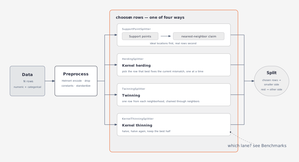
datasplit(splitter, data) runs the same five steps for every splitter; the sections that follow define the quantities involved. Given $N$ rows and ratio $= r$:
- Preprocess.
preprocessHelmert-encodes categorical columns in canonical level order, drops constant columns, and standardizes every remaining column to mean $0$ and variance $1$. The result is the matrix $X \in \mathbb{R}^{N \times p}$ on which every distance below is measured. - Size the smaller subset. $n = \operatorname{round}(\min(r, 1 - r)\,N)$.
datasplitraises anArgumentErrorif this leaves either subset empty. - Resolve the kernel.
resolvereplaces a:medianbandwidth with the median pairwise distance of the standardized rows; a numeric bandwidth andEnergyKernelpass through unchanged. The splitter carrying the resolved kernel is stored asresult.method. - Choose $n$ rows that represent all $N$. This is where the splitters differ and what the next four sections are about.
SupportPointSplitterfirst places $n$ free points._initial_pointsdraws $n$ rows of $X$ without replacement and jitters each by $10^{-3}$ of its column range;support_pointsthen moves the points to minimize the discrepancy between $\{\xi\}$ and $\{x\}$, by the MM update underEnergyKernelor by projected gradient descent underGaussianKernel. The optimized points are locations, not rows, soselect_nearestfinally rounds each one to its nearest unclaimed data row.HerdingSplitterskips the free points:herdpicks rows of $X$ directly, one greedy selection at a time.
- Label the two subsets. The $n$ chosen rows are the test set when $r \le 1/2$ and the training set otherwise; the remaining $N - n$ rows form the other side.
SplitResultcarries both index vectors together withconvergedanditerations(MM sweeps or gradient steps for support points; the number of selections, $n$, for herding).
Every random draw in these steps (the initial sample, the stochastic kappa subsets, and the sample behind :median) comes from the splitter's rng, so a fixed rng reproduces the split exactly. HerdingSplitter draws nothing beyond :median, which is why it is deterministic for a numeric kernel.
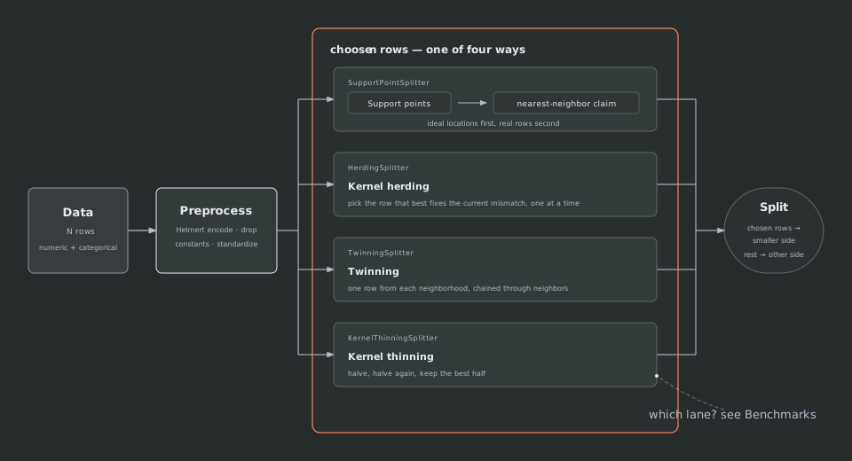
The figure summarizes the five steps. The Preprocess box stands for steps 1-3. The upper lane is SupportPointSplitter, with the two halves of step 4 as separate boxes: the highlighted support-point optimization, then the nearest-neighbor claim. The dashed lower lane is HerdingSplitter, which replaces both halves of step 4 by one greedy selection. Both lanes end in step 5.
splitquality(data, result) closes the loop. It repeats step 1 on the original data and evaluates the same discrepancy, energy distance or MMD², between the resulting train and test rows; for large data it does so through the Estimators below rather than exactly.
Energy distance and support points
Under EnergyKernel, the discrepancy step 4 minimizes (and splitquality reports) is the energy distance. Between two samples it is (Székely & Rizzo)
\[\mathrm{ED}(X, Y) = \frac{2}{|X||Y|} \sum_{x \in X} \sum_{y \in Y} \|x - y\| - \frac{1}{|X|^2} \sum_{x, x' \in X} \|x - x'\| - \frac{1}{|Y|^2} \sum_{y, y' \in Y} \|y - y'\|.\]
energydistance evaluates this V-statistic exactly by block-wise accumulation. With subsample = m it averages the statistic over random size-$m$ subsets; because the within-sample terms keep the zero diagonal, that estimate carries a positive bias of order $1/m$ and is meant for comparing splits, not as an absolute value.
Support points (Mak & Joseph, 2018) minimize $\mathrm{ED}(\{\xi\}, \{x\})$ over the point locations. The objective is minimized by majorization-minimization: at iteration $t$ every point moves to
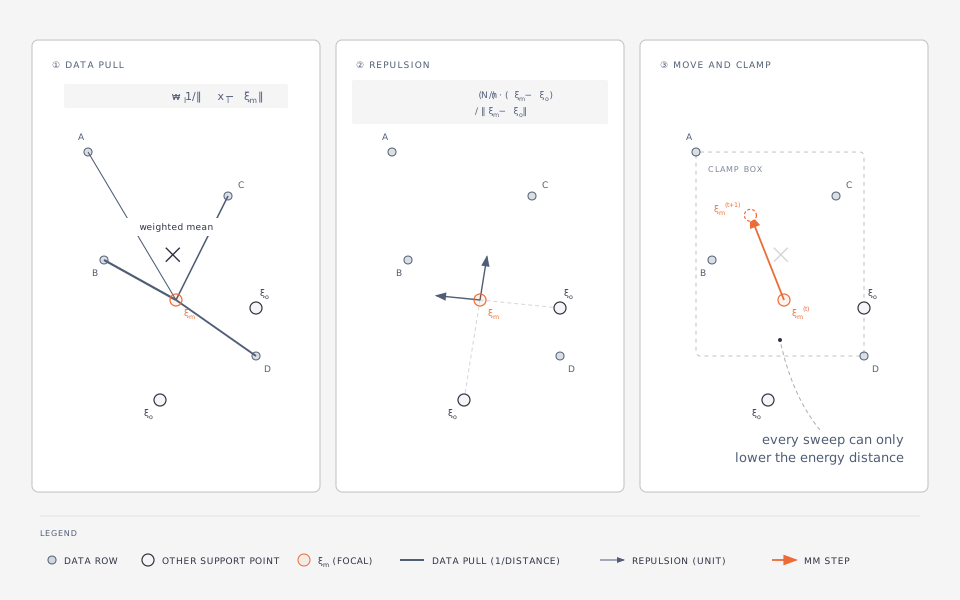
\[\xi_m^{(t+1)} = \frac{\displaystyle \frac{N}{n} \sum_{o \ne m} \frac{\xi_m^{(t)} - \xi_o^{(t)}}{\|\xi_m^{(t)} - \xi_o^{(t)}\|} + \sum_{l=1}^{N} \frac{x_l}{\|x_l - \xi_m^{(t)}\|}} {\displaystyle \sum_{l=1}^{N} \frac{1}{\|x_l - \xi_m^{(t)}\|}},\]
clamped to the data's bounding box. Each sweep decreases the energy distance monotonically (support_points(::EnergyKernel, …); the sweep is _mm_sweep!). With kappa $= \kappa < N$ the stochastic variant of Joseph & Vakayil (2022) uses a fresh random subset of $\kappa$ rows per iteration and blends the update with a running average whose weight $n_0 / (t + n_0)$, $n_0 = 0.2\,n$, decays with $t$. Iteration stops when the largest squared displacement of any point falls below tolerance.
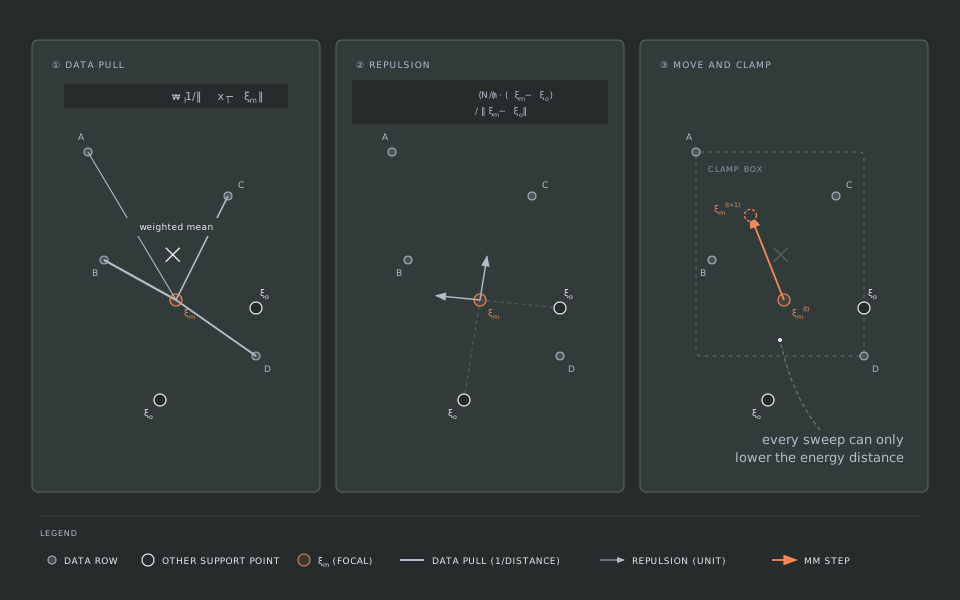
The update is a weighted mean of the data rows, each weighted by the inverse of its distance to $\xi_m$, plus a repulsion term divided by the same total weight: $N/n$ times one unit vector per other support point, pointing away from it. The figure splits one step for a single point $\xi_m^{(t)}$ (orange) into three panels of the same scene. Data pull: each grey line joins the point to a data row and its thickness is that row's weight $1/\|x_l - \xi_m\|$, so near rows are drawn heavy and far rows thin, and the × marks the resulting weighted mean. Repulsion: one arrow per other support point $\xi_o$, all of equal length, each the unit vector pointing away from $\xi_o$ and scaled by $N/n$. Move and clamp: the orange arrow is the sum of both terms, the move to $\xi_m^{(t+1)}$, and the dashed rectangle is the bounding box to which the result is clamped.
Maximum mean discrepancy and the Gaussian kernel
Under GaussianKernel, step 4 minimizes the squared maximum mean discrepancy instead, and support_points uses projected gradient descent on full data and the Gaussian MM sweep described below in stochastic mode. For a kernel $k$ the squared maximum mean discrepancy (Gretton et al.,
- between two samples is
\[\mathrm{MMD}^2(X, Y) = \frac{1}{|X|^2} \sum_{x, x'} k(x, x') + \frac{1}{|Y|^2} \sum_{y, y'} k(y, y') - \frac{2}{|X||Y|} \sum_{x, y} k(x, y).\]
mmd evaluates it (block-wise, with the same optional subsampling and the same bias caveat as energydistance). With $k(u, v) = -\|u - v\|$ this is the energy distance, which is why mmd covers both EnergyKernel and GaussianKernel.
GaussianKernel(σ) uses $k(u, v) = \exp\!\left(-\|u - v\|^2 / 2\sigma^2\right)$. Support points under it minimize, up to a constant,
\[f(\xi) = \frac{1}{n^2} \sum_{i,j} k(\xi_i, \xi_j) - \frac{2}{nN} \sum_{i,l} k(\xi_i, x_l), \qquad \nabla_{\xi_m} f = \frac{2}{n^2} \sum_{j \ne m} \nabla_u k(\xi_m, \xi_j) - \frac{2}{nN} \sum_{l} \nabla_u k(\xi_m, x_l),\]
with $\nabla_u k(u, v) = -k(u, v)\,(u - v)/\sigma^2$. The optimizer (support_points(::GaussianKernel, …)) takes projected gradient steps $\xi_{\text{new}} = \operatorname{clamp}(\xi - t \nabla f)$ where $t$ is chosen by Armijo backtracking on the projected step, $f(\xi_{\text{new}}) \le f(\xi) - 10^{-4}\, \langle \nabla f, \xi - \xi_{\text{new}} \rangle$; the objective therefore never increases across accepted steps.
The gradient carries $1/n^2$ and $1/(nN)$ factors whose magnitude varies enormously with $n$ and $N$, so the first trial step (_first_step) is scale-aware rather than a fixed constant: $t_0 = 0.1\,\bar w / \max_m \|\nabla_m f\|$, with $\bar w$ the median per-dimension data range, making the first move a tenth of the data scale regardless of $n$, $N$. Later iterations warm-start from twice the previous accepted step.
Convergence never fires before the second iteration, and then when either the largest squared displacement is below tolerance or the relative objective decrease $|f_{t-1} - f_t| / \max(|f_t|, 10^{-12})$ is below rtol (default $10^{-8}$); f here is the shifted objective above, which omits the constant data self-term and is bounded in $[-1, 1]$ for a Gaussian kernel, so rtol acts as an absolute-in-effect tolerance rather than a tolerance on the (orders-of-magnitude smaller) true MMD².
With kappa below the number of rows, the Gaussian kernel switches to a majorization–minimization sweep of the energy sweep's shape (support_points(::GaussianKernel, …) dispatches on kappa; the sweep shares the internal loop that also implements EnergyKernel's stochastic mode). The data term $-k(\xi, x)$ is concave in $\|\xi - x\|^2$, so its tangent at the current point is an upper bound whose minimizer is the mean-shift step (Fukunaga & Hostetler, 1975): the kernel-weighted mean of the data. The repulsion $k(\xi_i, \xi_j)$ is bounded above by its quadratic $L$-smooth majorizer, $L$ here the Lipschitz constant of the repulsion's gradient, with $L = 2e^{-3/2}/\sigma^2$, the largest Hessian eigenvalue of a Gaussian, split evenly over the two points. Per point, with $s_0 = \sum_l k(\xi_m, x_l)$, $s_1 = \sum_l k(\xi_m, x_l)\,x_l$, $r_0 = \sum_{j \ne m} k(\xi_m, \xi_j)$, $r_1 = \sum_{j \ne m} k(\xi_m, \xi_j)\,\xi_j$,
\[A = \frac{s_0}{N\sigma^2}, \quad \mathrm{ms} = \frac{s_1}{s_0}, \quad \mathrm{rep} = \frac{r_0\,\xi_m - r_1}{n\sigma^2}, \quad B = \frac{4(n-1)e^{-3/2}}{n\sigma^2}, \qquad \xi_m \leftarrow \operatorname{clamp}\!\left(\frac{A\,\mathrm{ms} + B\,\xi_m + \mathrm{rep}}{A + B}\right).\]
(In stochastic mode, the only mode in which this sweep runs, $\kappa$ takes the place of $N$ in $A$: the sums run over the drawn rows.) $A + B > 0$ always, the sweep is one pass over the data and the point set, and on full data the objective never increases (the majorizer is tangent at the current points, so its minimizer cannot be worse). For large $n$ ($B$ approaches $4e^{-3/2}/\sigma^2 \approx 0.89/\sigma^2$ and $A \le 1/\sigma^2$) the attraction weight $A/(A+B)$ is at most about $0.53$, so a sweep moves a point at most about halfway to its mean-shift target; per iteration this descends less than a line search would, but an iteration costs a single pass, which is what makes the stochastic mode affordable. With $\kappa < N$ the sweep runs on a fresh subsample each iteration with the running-average blend of the energy path ($n_0 = 0.2n$); weights enter the data sums as $\hat w$, and a reference replaces the data rows, exactly as for EnergyKernel. Convergence is the displacement rule.
Full data keeps the Armijo path instead of this sweep because it measures better there: the sweep never reaches the displacement rule within the iteration cap and its selected rows are worse on uniform-5d at both sizes and on t3-3d at N = 1,000 (0.000156 vs 0.000118), level or better elsewhere. In kappa mode, where only the sweep is affordable, the selected-row MMD at N = 10,000 is within about 3% of Armijo's on normal-10d and t3-3d, about 29% higher on uniform-5d (0.000393 vs 0.000305), and about 10x higher on mixture-2d (5.47e-6 vs 5.6e-7, still about 2x below the random subset's 1.23e-5), while running 3.4-3.8x faster than the full-data sweep (see Design experiments). The design record (docs/superpowers/specs/2026-09-04-gaussian-mm-update-design.md) explains why the weighted mean-shift map of Belhadji, Sharp & Marzouk (2025) is not used as written: it optimizes the subset's weights too, and the package's selected subset is uniform.
When bandwidth = :median, $\sigma$ is the median pairwise distance over (a sample of) the standardized rows (Gretton et al., 2012), resolved once per datasplit and stored in result.method.kernel. A bandwidth far below the row spacing makes the objective flat: on full data the points barely move and Armijo's backtracking stalls at a tiny step; in kappa mode the displacement rule stops at the initial sample.
Kernel herding
HerdingSplitter replaces the place-then-round scheme of step 4 with a direct greedy selection: it builds the smaller subset row by row. With data $x_1, \dots, x_N$ and rows $s_1, \dots, s_T$ already selected, the next row is (Chen, Welling & Smola, 2010, Eq. 8, applied to the empirical distribution and restricted to unselected rows)
\[s_{T+1} = \arg\max_{x \notin \{s_1,\dots,s_T\}} \; \frac{1}{N} \sum_{l=1}^{N} k(x, x_l) \;-\; \frac{1}{T+1} \sum_{t=1}^{T} k(x, s_t).\]
Appending $x$ changes the MMD² between the selected rows and the data by
\[\Delta(x) = \frac{k(x,x)}{(T+1)^2} + \frac{2}{(T+1)^2} \sum_{t=1}^{T} k(x, s_t) - \frac{2}{(T+1)N} \sum_{l=1}^{N} k(x, x_l) + \text{const},\]
so for kernels with constant $k(x, x)$, namely the Gaussian kernel ($1$) and the energy kernel $k(u,v) = -\|u - v\|$ ($0$), the herding choice is exactly the greedy MMD² (energy-distance) minimizer. For the Gaussian kernel (a bounded feature map), the error $\mathcal{E}_T$ of Eq. (9) decreases as $O(1/T)$ (Proposition 1); for the energy kernel only the greedy-step equivalence with MMD²/energy-distance minimization above is claimed, not the $O(1/T)$ rate.
herd computes the exact data term once ($O(N^2)$) and maintains the running sum over selected rows in $O(N)$ per selection, for a total cost of $O(N^2 + nN)$; the procedure is deterministic for a numeric kernel.
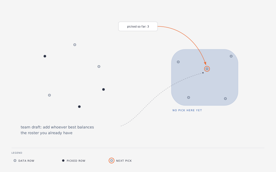
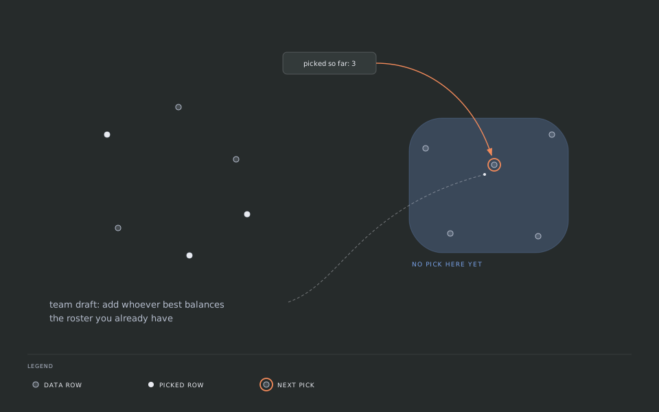
The figure shows one greedy step: three rows already selected (filled) all lie in the left cluster, so the data term of the right cluster is unmatched and the argmax above lands there (the ringed row).
Nearest-neighbor assignment
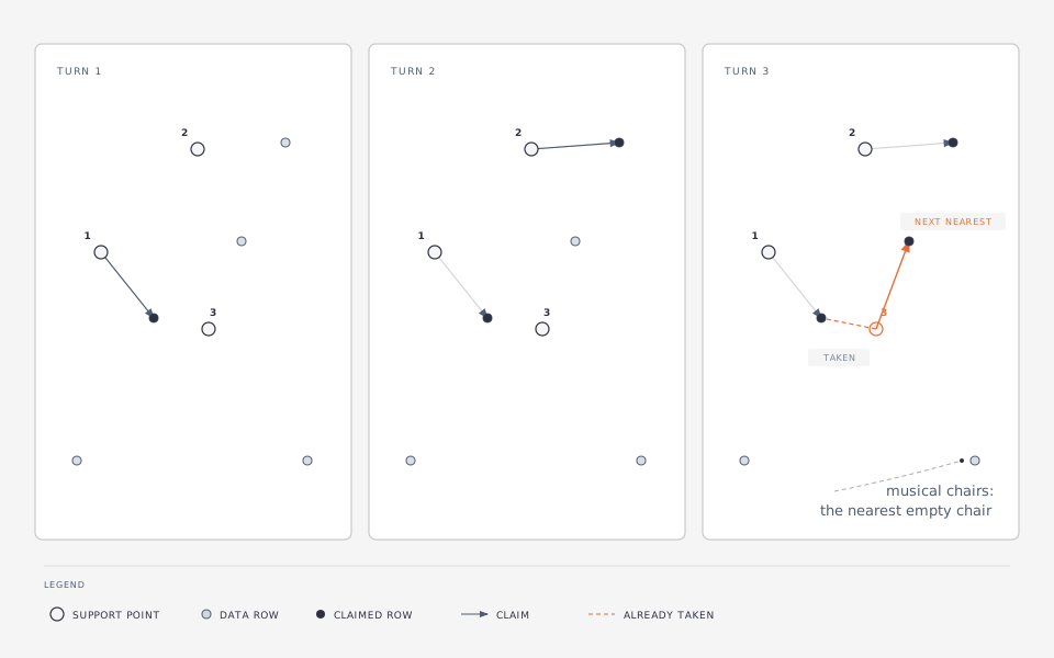
The last part of step 4 for SupportPointSplitter turns optimized locations into rows. Each support point, in order, claims its nearest not-yet-claimed data row (Joseph & Vakayil, 2022). select_nearest serves the queries from a k-d tree, doubling the neighbor count and retrying when every returned neighbor is already claimed. The claimed rows form the smaller subset.
Below 200 columns the k-d tree serves the query; from 200 on, a plain-matrix brute-force search does. The threshold sits where the two cross: the matrix search is within about 15% of the k-d tree at 200 columns and about three times faster at 768, while the k-d tree's width-specialized code costs a first-call compilation that grows with the width and stops finishing in practical time above a few thousand columns (see Matrix brute-force search).
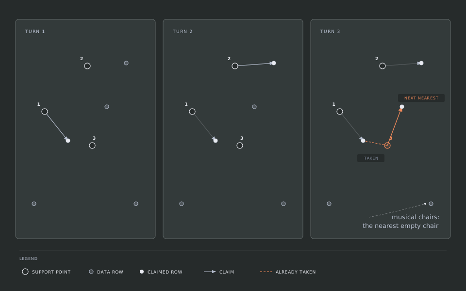
The figure shows three turns of the claim side by side. Hollow circles are support points numbered in claim order, grey circles are unclaimed rows, and filled circles are claimed rows. Points 1 and 2 take their nearest row in turns 1 and 2; in turn 3, point 3 (orange) finds its nearest row already claimed by point 1 (dashed line) and takes its second-nearest row instead (solid orange arrow).
This rounding step has a limitation: when the optimizer's displacement is below the spacing between data rows, as is typical in high dimension on standardized data, every point's nearest row is still its own starting row, so the claimed subset is exactly the initial random sample and the optimization has no effect on which rows are selected. Measured on the Benchmarks page. HerdingSplitter selects rows directly and has no rounding step, so it is unaffected.
Estimators
The optimizers in step 4 always work with the exact objective. Measuring a finished split is a separate matter: energydistance, mmd, and splitquality accept an estimator keyword that selects how the discrepancy above is computed. Which estimator/kernel combinations exist is expressed by method dispatch (a method per combination, never an if); an undefined combination raises an ArgumentError.
| estimator | energydistance (EnergyKernel) | mmd (GaussianKernel) |
|---|---|---|
Exact | yes, threaded | yes, threaded |
Subsample(m, repeats) | yes | yes |
RandomSlices(k) | yes | no |
RandomFeatures(D) | no | yes |
RandomSlices: the projection identity
For $\theta$ uniform on the unit sphere $S^{p-1}$ and any $u \in \mathbb{R}^p$,
\[\mathbb{E}_\theta\,|\langle \theta, u \rangle| = \kappa_p \|u\|, \qquad \kappa_p = \frac{\Gamma(p/2)}{\sqrt{\pi}\,\Gamma\!\left((p+1)/2\right)},\]
computed by sphere_constant via the recursion $\kappa_1 = 1$, $\kappa_2 = 2/\pi$, $\kappa_{p+2} = \kappa_p\,p/(p+1)$. The energy distance is linear in the pairwise norms, so with $u^\theta = X\theta$, $v^\theta = Y\theta$,
\[\mathrm{ED}(X, Y) = \kappa_p^{-1}\, \mathbb{E}_\theta\, \mathrm{ED}_1(u^\theta, v^\theta),\]
and RandomSlices(k) averages this over k directions drawn with rng (_sliced_energydistance). The one-dimensional energy distance $\mathrm{ED}_1$ is computed exactly from sorted projections (_ed1d): for a sorted sample $a_{(1)} \le \dots \le a_{(n)}$,
\[\sum_{i<j} (a_{(j)} - a_{(i)}) = \sum_i (2i - n - 1)\, a_{(i)}\]
gives the within-sample mean (_within_mean_abs), and the cross term $\sum_{i,j} |a_i - b_j|$ follows from prefix sums of one sorted sample and the ranks of the other (_cross_mean_abs), for a total cost of $O(k (n+m) \log(n+m))$.
RandomFeatures: random Fourier features
For the Gaussian kernel $k(x,y) = \exp(-\|x-y\|^2/2\sigma^2)$, with $\omega_j \sim \mathcal{N}(0, \sigma^{-2} I_p)$ and $b_j \sim U[0, 2\pi]$ (Rahimi & Recht, 2007),
\[z(x) = \sqrt{2/D}\,\big[\cos(\omega_j^\top x + b_j)\big]_{j=1}^{D}, \qquad \mathbb{E}\big[z(x)^\top z(y)\big] = k(x, y),\]
drawn once per call from rng as FourierFeatureMap. RandomFeatures(D) estimates squared MMD as $\|\bar z_X - \bar z_Y\|^2$ with $\bar z_X = \frac{1}{n}\sum_i z(x_i)$ (_rff_mmd, _feature_mean), an unbiased estimator of the V-statistic, cost $O((n+m)Dp)$.
Exact: threaded
_mean_pairwise and _mean_kernel split their block loop over row-block pairs across n_threads spawned tasks, each writing disjoint entries of a preallocated accumulator that is then summed in a fixed pair order, so the result is identical for every thread count, not just numerically close.
Automatic rule for splitquality
estimator = nothing (the default) selects Exact() when the total row count is at most exact_threshold (20,000), and otherwise the fallback chosen by the Estimator selection experiment on the Design experiments page (_fallback_estimator).
Why herding stays exact
RandomSlices/RandomFeatures give an unbiased data term for kernel herding too, but measurement rejected them: every candidate row's estimate shares the same random directions or features, so the estimator noise is correlated across rows, and the greedy argmax follows that correlated noise into a direction-dependent region of the data rather than averaging it out. At feasible budgets the selected subset was worse than a random subset. See Approximate herding data terms (rejected) on the Design experiments page for the table. HerdingSplitter's data term (_data_term) therefore stays exact only.
Optimal split ratio
Step 2 takes ratio as given; optimal_split_ratio is one way to choose it. For a linear model with $p$ parameters (intercept included), Joseph (2022, Eq. 11) gives the test fraction that minimizes the variance of the fitted model:
\[\gamma^* = \frac{1}{\sqrt{p} + 1}.\]
optimal_split_ratio(x, y) takes $p$ as the number of encoded predictor columns plus one.
References
- Belhadji, A., Sharp, D., & Marzouk, Y. (2025). Weighted quantization using MMD: From mean field to mean shift via gradient flows. arXiv:2502.10600.
- Chen, Y., Welling, M., & Smola, A. (2010). Super-Samples from Kernel Herding. UAI, 109-116.
- Dwivedi, R., & Mackey, L. (2022). Generalized Kernel Thinning. ICLR.
- Dwivedi, R., & Mackey, L. (2024). Kernel Thinning. Journal of Machine Learning Research, 25(152), 1-77.
- Fashing, M., & Tomasi, C. (2005). Mean shift is a bound optimization. IEEE Transactions on Pattern Analysis and Machine Intelligence, 27(3), 471-474.
- Fukunaga, K., & Hostetler, L. (1975). The estimation of the gradient of a density function, with applications in pattern recognition. IEEE Transactions on Information Theory, 21(1), 32-40.
- Gretton, A., Borgwardt, K. M., Rasch, M. J., Schölkopf, B., & Smola, A. (2012). A Kernel Two-Sample Test. JMLR, 13, 723-773.
- Joseph, V. R. (2022). Optimal Ratio for Data Splitting. Statistical Analysis and Data Mining, 15(4), 531-538.
- Joseph, V. R., & Vakayil, A. (2022). SPlit: An Optimal Method for Data Splitting. Technometrics, 64(2), 166-176.
- Mak, S., & Joseph, V. R. (2018). Support points. The Annals of Statistics, 46(6A), 2562-2592.
- Rahimi, A., & Recht, B. (2007). Random Features for Large-Scale Kernel Machines. NIPS, 20.
- Shetty, A., Dwivedi, R., & Mackey, L. (2022). Distribution Compression in Near-Linear Time. ICLR.
- Székely, G. J., & Rizzo, M. L. (2013). Energy statistics: A class of statistics based on distances. Journal of Statistical Planning and Inference, 143(8), 1249-1272.
- Vakayil, A., & Joseph, V. R. (2022). Data Twinning. Statistical Analysis and Data Mining, 15(5), 598-610.
Weighted samples
Every quantity above is defined for the empirical distribution of the data, in which each row has mass $1/N$. Passing weights (one non-negative entry per row, positive sum) replaces it by the weighted empirical distribution $P_w = \sum_i \bar w_i\, \delta_{x_i}$ with $\bar w_i = w_i / \sum_l w_l$; the selected subset itself stays uniformly weighted. Nothing else changes: the procedure runs the same five steps, and weights = nothing (the default) is the unweighted case. A constant weight vector is turned into nothing after validation, so uniform weights take the same unweighted path and reproduce it exactly.
Which steps read the weights:
- Preprocess.
preprocess(data, weights)standardizes with the weighted mean $\mu_j = \sum_i \bar w_i x_{ij}$ and the unbiased weighted variance $\sigma_j^2 = \sum_i \bar w_i (x_{ij} - \mu_j)^2 / (1 - \sum_i \bar w_i^2)$, which is the usual $n - 1$ denominator for uniform weights. - Resolve the kernel. A
:medianbandwidth is the median pairwise distance over rows drawn in proportion to the weights. This only changes the resolved bandwidth for datasets above 1000 rows; below that every row enters the median and the weights do not change it. - Choose $n$ rows. The data terms carry the weights:
- The energy distance between the support points and $P_w$ is $\frac{2}{n} \sum_{m,i} \bar w_i \|\xi_m - x_i\| - \frac{1}{n^2}\sum_{m,o} \|\xi_m - \xi_o\| - \sum_{i,k} \bar w_i \bar w_k \|x_i - x_k\|$, and MMD² is the same expression with kernel values in place of negated distances. The MM update of Mak & Joseph (2018) and the projected gradient keep their form with $\bar w_i$ multiplying every data term, so the MM step is still monotone.
- Kernel herding's data term becomes $\sum_l \bar w_l\, k(x, x_l)$.
splitquality(data, result; weights) compares the weighted train rows with the weighted test rows, each side's weights rescaled to sum one, and energydistance/mmd accept weights_x and weights_y for the two samples; every DiscrepancyEstimator has a weighted form (Subsample rescales the weights of the rows it draws, RandomSlices uses the weighted one-dimensional energy distance on each projection, and RandomFeatures uses weighted feature means). Weights proportional to duplication counts are equivalent to duplicating rows, up to the common column rescaling of the weighted standardization, which changes nothing under EnergyKernel or a :median bandwidth but does matter for a fixed numeric Gaussian bandwidth, which is what the tests check. How stochastic kappa subsampling combines with weights was decided by the experiment on the Design experiments page.
Reference distribution and selectrows
By default the chosen rows approximate the distribution of the data they are drawn from. Passing reference (a second sample with the same columns, optionally weighted by reference_weights) makes them approximate the reference instead, while the candidates stay the rows of data. Only two steps of the procedure change:
- Step 1: Preprocess. The transform is fit on the reference and applied to both sets: categorical levels are the union of both sets' levels, and the reference's mean and scale (weighted forms with
reference_weights) standardize every row. Columns that are constant on the reference but vary in the data are kept, not dropped: they are centered at the reference's value and scaled by the data's spread, so candidates away from that value are penalized. Columns constant on both sets are dropped. - Step 3: Resolve the kernel. A
:medianbandwidth is resolved on the encoded reference.
Step 4 keeps its rules with the reference as the target measure: the data term of the energy distance or MMD² runs over the $M$ reference rows $r_1, \dots, r_M$ with weights $\bar v_l$, the support points start at rows of data and are rounded to rows of data, and kernel herding's data term becomes $\sum_l \bar v_l\, k(x, r_l)$ for every candidate $x$. weights for the data cannot be combined with reference. Support points are clamped to the bounding box of data, so a reference lying outside that box cannot be matched beyond the box, and monotone descent is guaranteed only while the box does not bind.
selectrows(splitter, data, n; ...) runs the same steps and returns the n chosen row indices without forming a partition; datasplit is selectrows with n set by ratio plus the complement, and result.selected names the side that holds the chosen rows. splitquality(data, result; reference) then measures the chosen rows against the reference, which is the quantity the splitter minimized.
Twinning and multiplets
TwinningSplitter (Vakayil & Joseph, 2022) replaces steps 3 and 4 of the procedure: no kernel to resolve, no optimizer, and no separate nearest-neighbor assignment. It works directly on the standardized rows, and its objective is still the energy distance: by Proposition 1 of the paper, the energy distance between the smaller twin and the whole data, the SPlit objective, is $(1 - \gamma)^2$ times the energy distance between the two twins, so minimizing the gap between the twins minimizes the SPlit objective.
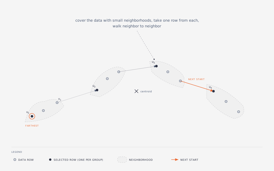
Given $n$ rows to select, twinning covers the data with $n$ disjoint groups and selects one row per group (Algorithm 1). Below, $r$ denotes the group size, $N \div n$; it is not the split ratio from step 2, which this section does not use again.
- Start at $u_1$: with
start = :farthest(the default) the row farthest from the centroid, with:randoma row drawn fromrng, or a given row index. - Group $i$ is $u_i$ together with its $r_i - 1$ nearest ungrouped neighbors, ordered by distance; let $v_i$ be the farthest of them.
- $u_{i+1}$ is the ungrouped row nearest to $v_i$.
The selection is $u_1, \dots, u_n$. Every unselected row sits in a small neighborhood of a selected one, and the groups form a chain of adjacent neighborhoods, which is what keeps the two sides close in energy distance (paper, Section 3.1). Nearest neighbors come from a k-d tree in which grouped rows are masked; the tree is rebuilt on the remaining rows whenever more than half of its rows are masked, so the average cost stays $O(pN \log N)$ (paper, Eq. 12). Above a dimension fixed by measurement (see Design experiments) the rows are scanned by brute force instead. The procedure is serial and deterministic given the data and a non-random start; SplitResult.iterations is the number of groups.
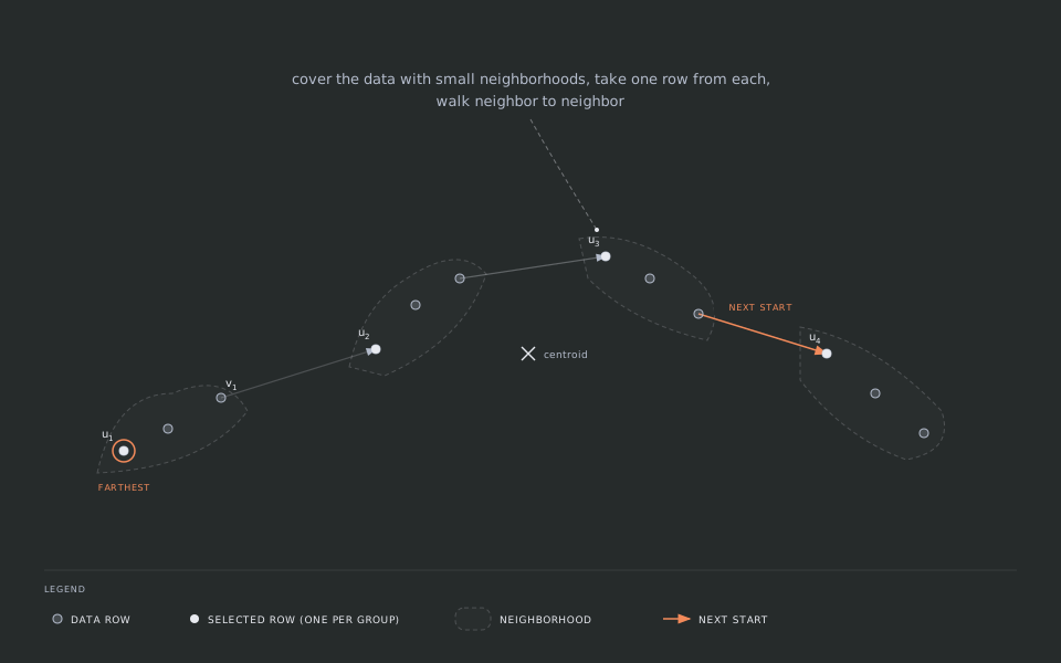
The figure draws Algorithm 1 with $r = 3$: the × is the centroid, $u_1$ (ringed) is the row farthest from it, each dashed hull is one group of $r$ rows, and each arrow runs from $v_i$, the farthest member of a group, to $u_{i+1}$, the nearest ungrouped row. Filled circles are the selected rows $u_1, \dots, u_4$.
Differences from the paper. The paper assumes $1/\gamma = r$ is an integer and takes $n = \lceil \gamma N \rceil$, letting the last group absorb the remainder. SPlit.jl keeps the generic rule ($n$ from ratio in datasplit, or the caller's $n$ in selectrows) and sets $r = \lfloor N/n \rfloor$, with the $N - rn$ leftover rows forming groups of $r + 1$ spread evenly along the chain; when $N = rn$ the two coincide. weights and reference are not defined for twinning and raise an ArgumentError.
Multiplets
multiplet(splitter, data, k; strategy) returns $k$ folds that partition the rows, each distributed like the whole data (paper, Section 5), with sizes differing by at most one:
:sequential(S1, default): select $\lfloor N/k \rfloor$ rows with the splitter, then $\lfloor N'/(k-1) \rfloor$ of the remaining $N'$ rows, and so on; the last fold is what remains. Works with every splitter and re-fits the preprocessing on the remaining rows each time.:halving(S2): split every part in half repeatedly; $k$ must be a power of two. Works with every splitter.:single(S3): one twinning run with groups of at least $k$ rows; fold $j$ collects the $j$-th member of every group.TwinningSplitteronly, a single pass, and the paper measures it slightly behind S1 and S2.
The paper judges multiplets by the largest energy distance between any fold and the whole data; the tests check that it is below the random-partition average for all three strategies.
Kernel thinning
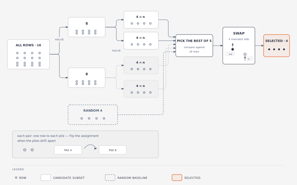
KernelThinningSplitter (Dwivedi & Mackey, 2022, 2024) selects rows directly, like herding, but by a randomized halving scheme with a non-asymptotic MMD guarantee. It replaces steps 3 and 4 of the procedure and keeps the kernel of step 2: with the target kernel $k$ (the energy kernel by default), the split kernel of the papers is $k$ itself ("target kernel thinning").
- Kernel halving. Rows are visited two at a time in a random order. For the pair $(x, x')$ let $f = k(x, \cdot) - k(x', \cdot)$, $b^2 = \|f\|_k^2 = k(x,x) + k(x',x') - 2k(x,x')$, and $\alpha = \sum_{z \in S_2} f(z) - \sum_{z \in S_1} f(z)$ over the two halves built so far. One row goes to each half; the assignment is swapped with probability $\min(1, \tfrac12 (1 - \alpha/a)_+)$, where the threshold $a$ is updated from $b$ and a running parameter $\sigma$ so that the halving stays balanced with probability at least $1 - \delta_{\mathrm{step}}$, for a per-step failure probability $\delta_{\mathrm{step}}$ fixed by the caller.
- KT-SPLIT. With $m = \lfloor \log_2 (N/n) \rfloor$, the first $L = n 2^m$ rows of the shuffle ($L$ here the KT block size, not the Lipschitz constant of the Gaussian-kernel section above) are halved $m$ times, giving $2^m$ candidate subsets of size $n$; every halving at every level shares the same $\delta_{\mathrm{step}} = \delta / (mL)$, the papers' per-point $\delta_i = \delta/L$ (
delta, default $0.5$) applied as $\delta_i/m$ at each of the $m$ levels. - KT-SWAP. A uniform random subset of size $n$ joins the candidates; the one with the smallest $\frac{1}{n^2}\sum_{a,b \in S} k(a,b) - \frac{2}{n}\sum_{a \in S} d(a)$ (the MMD² to the target measure up to a constant, with $d(a) = \sum_l \bar v_l k(a, r_l)$ the data term of step 4 of kernel herding) is refined by one pass over its positions, each replaced by the row outside the subset that lowers the objective most, if any.
The result is never worse than the random baseline, and each KT-SPLIT candidate carries the papers' $O(\sqrt{\log n / n})$ MMD bound against the empirical measure of the $L$ rows that entered KT-SPLIT (all $N$ rows when $N/n$ is a power of two); the KT-SWAP step then targets the full data. The cost is $O(L^2)$ kernel evaluations for the halvings, $O(N^2)$ for the data term and $O(nN)$ for the swap pass, all threaded: the same class as herding. The near-linear variant of the papers, Compress++, removes the two $O(N^2)$ terms when $n \ll N$; it is the next section.
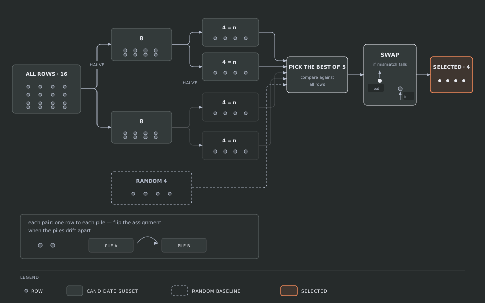
The figure follows the three steps with $N = 16$ and $n = 4$, so $m = 2$: two rounds of kernel halving produce the $2^m = 4$ candidates, the dashed box is the uniform random subset that joins them, and KT-SWAP picks the best of the five and refines it by one swap pass. The inset is one step of kernel halving: a pair of rows, one to each half, with the probabilistic flip that keeps the halves balanced.
Differences from the paper. The papers thin $N$ rows to $\lfloor N/2^m \rfloor$; here $n$ is set by ratio (or the caller) and the $N - L$ rows left out of KT-SPLIT still enter KT-SWAP as candidates and through the target measure; the two agree when $N/n$ is a power of two. Swap candidates exclude rows already selected, so the split is a set of distinct rows. weights and reference change the KT-SWAP objective only (the target measure $P_w$ or $P_R$ of the sections above); the halvings always run on the unweighted candidate rows. For $n > N/2$, selectrows returns the complement of a kernel-thinning selection of the $N - n$ rows not chosen: the two halves of kernel halving are symmetric, and for a subset $S$ of size $n_c \le N/2$ with complement $C$, the mean-embedding identity $\mu_N = (n_c/N)\mu_S + ((N-n_c)/N)\mu_C$ gives $\mathrm{MMD}(C, P_N) = (n_c/(N-n_c)) \cdot \mathrm{MMD}(S, P_N) \le \mathrm{MMD}(S, P_N)$, so the complement is at least as close to the data as the thinned set (this identity is only approximate under weights or reference).
Compress++
For $n \ll N$ the $O(N^2)$ cost of kernel thinning is dominated by the first halving of all $N$ rows and by the data term. Compress++ (Shetty, Dwivedi & Mackey, 2022) avoids both: with $g$ an oversampling parameter (defined below), it never halves more than about $2^{g+1}\sqrt{N}$ rows at once.
- Compress. A random permutation of the rows is split into four consecutive parts, each part is compressed recursively (sequences of at most $4^g$ rows are returned as they are), the four results are concatenated and halved. The halving is kernel thinning of the block of $\ell$ rows to $h = \lfloor \ell/2 \rfloor$ rows, kept with probability $h/\ell$; otherwise the complement is kept, trimmed by one row chosen at random when $\ell$ is odd. Every row of the block is then kept with probability exactly $h/\ell$ (a fair coin for even $\ell$), so each halving is unbiased for the block's mean embedding. The output has about $2^g \sqrt N$ rows.
- Thin. Kernel thinning then selects $n$ rows from the compressed set, with the compressed rows as its data term and swap candidates.
KernelThinningSplitter(compress = :auto) runs Compress++ when the target measure is the data itself and the estimated cost $4^g N (4\log_4 N + 1)$ is below plain kernel thinning's $1.5 N^2$, with $g = \max(4, \lceil \log_2(2n/\sqrt N) \rceil)$ (the paper's experiments use $g = 4$; the second term keeps the compressed set at about $2n$ rows). The rule does not fire at the default 20% split ratio, so datasplit with the default splitter is unchanged; it can fire below roughly a 10% ratio once $N \ge 10^4$ (up to $n = 800$ at $N = 10^4$, 10,100 at $N = 10^5$ and 64,000 at $N = 10^6$), which is where selectrows and multiplet usually sit. Pass compress = :never to keep the plain path there; :always forces Compress++. The rule was checked against wall time and quality in Compress++ cost rule: where it fires, Compress++ is 1.3-6.9x faster in six of seven measured cells (a tie in the seventh) at a 3-16% energy-distance cost.
Differences from the paper. The halving algorithm is kernel thinning of the block (split and swap), the failure probability is split evenly over the halvings and the final thinning, the four parts may differ in size by one row, and $g$ grows with $n$ so that any $n$ can be requested. Compress++ is not defined for weights or reference; :auto falls back to plain kernel thinning there.
Skipping preprocessing
standardize = false on datasplit, selectrows, multiplet, splitquality, and compare skips step 1 entirely: a numeric matrix (or vector, as one column) is used as it is, with no centering, scaling, or constant-column removal, and a reference is used the same way. Use it when the rows already live in the geometry you want to preserve, such as cosine-normalized embeddings, where per-column standardization would distort angles. A DataFrame needs the encoding of step 1 and is rejected with standardize = false.
The LLM data-selection guide is the worked workflow for that case.